Charge Limiters for Increasing the Battery Life of Plugged-In Laptops on macOS

When using a MacBook primarily plugged into a charger, it's often beneficial to limit the battery charge to around 80%. Charging up to 100% regularly can lead to increased wear on the battery, reducing its long-term lifespan. By keeping the battery charge capped at 80%, you can reduce the stress on the battery, which helps to maintain its health over time, especially for devices that are always connected to power.

A popular open-source charge limiter for macOS that can help manage this is:

AlDente Charge Limiter. This tool offers an easy way to set a charge limit, allowing you to configure your MacBook to charge only up to your desired level (e.g., 80%).

How to Abbreviate Author Names in IEEEbib.bst

When working with IEEE references in BibTeX, the IEEEbib.bst style is commonly used for IEEE conferences and journals. However, by default, this style formats author names in full (e.g., "John Smith" rather than "J. Smith"). If you'd like to abbreviate the first name to its initial, you can modify the IEEEbib.bst file by adjusting the way author names are formatted. For that you just need to modify the format.names function.

Find the format.names function in the IEEEbib.bst file. It looks like this:

FUNCTION {format.names}

{ 's :=

  #1 'nameptr :=

  s num.names$ 'numnames :=

  numnames 'namesleft :=

    { namesleft #0 > }

    { s nameptr "{ff~}{vv~}{ll}{, jj}" format.name$ 't :=

      nameptr #1 >

{ namesleft #1 >

    { ", " * t * }

Just replace {ff~} with {f.~} in the 7th line to abbreviate first names, i.e.

    { s nameptr "{f.~}{vv~}{ll}{, jj}" format.name$ 't :=

Slow SSHFS transfer speeds under OSX

If you’ve noticed that SSHFS transfers are much slower (several times slower) than SCP on macOS, you're not alone. This issue seems to be tied to how macFUSE and SSHFS interact, particularly around I/O block size. A detailed discussion about the root cause of this problem can be found in a GitHub issue thread.

The good news is that in the tread it is also proposed a fix: increase the I/O block size. By setting it to 1MB (-o iosize=1048576), I was able to significantly speed up transfers with just a small 10% overhead.

I applied this change by adding it to my ~/.zshrc (or ~/.bashrc):

     alias sshfs='sshfs -o iosize=1048576'

It's a quick win if you rely on SSHFS for remote file systems!

Brighten an \includeimage image in LaTeX Using decodearray without modifying the file

You can adjust the brightness of \includegraphics images in LaTeX without editing them!

The decodearray option in the graphicx package allows you to modify the appearance of images directly within your document.
This is especially useful if you need to tweak image brightness directly in your document without relying on external image editing tools.
The decodearray feature relies on PDF features supported by modern LaTeX engines  such as LuaLaTeX or XeLaTeX. 

\documentclass{article}
\usepackage{graphicx}
\begin{document}

% Original RGB image
\section*{Original Image}
\includegraphics[width=0.5\textwidth]{example-image.jpg}

% Brightened image using decodearray
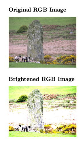
\section*{Brightened RGB Image}
\includegraphics[width=0.5\textwidth, decodearray={0.2 0.5   0.2 0.5   0.2 0.5}]{uiskentuie_standing_stone.png}

\end{document}

In the example decodearray={0.2 0.5    0.2 0.5    0.2 0.5} maps the original range [0, 1] for each one of the three RGB channels to a narrower, brighter range [0.2, 0.5].

source: https://tex.stackexchange.com/questions/29227/can-includegraphics-be-used-to-change-an-image-color/150219#150219

Running HTTPS and SSH over the same port with SSLH

Do you need to access your network services from remote locations but are blocked by firewalls or other
access restrictions? You might want to try SSLH, a powerful open-source tool that enables you to run multiple network services over a single port. This allows you to bypass firewalls and access your network services from anywhere. Here will show you how to use SSLH to run both HTTPS and SSH on the same port, but SSLH also supports HTTP and OpenVPN. 

Installing SSLH

SSLH is available in most Linux distributions' package managers, so installation is straightforward. You can install SSLH using the following command:

$ sudo apt-get install sslh

Configuring SSLH

Once SSLH is installed, you need to configure it to run both HTTPS and SSH on the same port. The configuration file for SSLH is usually located at /etc/default/sslh. In the configuration below SSLH listens on all available network interfaces on port 443, and it proxies SSH to port 22 of localhost and HTTPS to port 2443 of localhost. 

DAEMON_OPTS="-u sslh -p 0.0.0.0:443 -s 127.0.0.1:22 -l 127.0.0.1:2443 -P /var/run/sslh.pid"

RUN=yes

Before restarting SSLH, make sure to configure your web server to listen to 2443 instead of 443. Then, restart SSLH with

$ /etc/init.d/sslh start

Testing SSLH

To test SSLH, you can try accessing both the HTTPS and SSH services through the SSLH port. For example, to access HTTPS, open a web browser and navigate to https://<your-server-address>:443. To access SSH, open a terminal and use the ssh command  ssh your-server-address -p 443. 

source: https://memo-linux.com/sslh-https-et-ssh-sur-le-meme-port/, https://github.com/yrutschle/sslh

Reset Windows passwords with chntpw using a Linux Live USB

Have you ever forgotten your Windows login password and been locked out of your own computer?
There is a way to reset your Windows password using a Linux Live USB drive and a tool called chntpw. Here, we will show how.

Step 1: Create a Linux Live USB drive

First, you'll need to create a Linux Live USB drive. You can use any Linux distribution that includes the chntpw package. We will be using Ubuntu:

• Download the Ubuntu ISO file from the official website.
• Burn the ISO file to a USB drive using a tool like Rufus or Etcher.
• Boot your computer from the USB drive.

Step 2: Install chntpw

Once you have booted into the Linux Live USB, you'll need to install the chntpw package. To install chntpw, open a terminal and run the following command:

sudo apt install chntpw

Step 3: Mount the Windows partition

Next, you'll need to mount the Windows partition that contains the password database. In the terminal, navigate to the directory where the Windows partition is mounted. This will typically be the Windows/System32/config/ directory.

cd ~/winmount/Windows/System32/config/

Step 4: List the Windows users

Now, list the Windows users stored in the password database by running the following command:

sudo chntpw -l SAM

This will display a list of Windows users along with their corresponding User IDs (UIDs).

Step 5: Reset the Windows password

Finally, you can reset the password for a specific Windows user by running the interactive command:

sudo chntpw -i SAM

This will launch a menu where you can select the user whose password you want to reset and also unlock accounts. Follow the prompts to reset the password. Then reboot into Windows.

Sources: https://doc.ubuntu-fr.org/tutoriel/chntpw; https://ostechnix.com/reset-windows-password-with-linux-live-cd/

Make a bootable Linux/Ubuntu live USB drive on OS X

We'll see how to create a bootable Linux/Ubuntu USB drive, from an ISO image, on OS X using command line commands.

Step 1: Download the Ubuntu Image

The first step is to download the Ubuntu image from the official website. Live CD images allow to run Ubuntu without installing it. Here, we'll use an old Ubuntu 16 image from https://releases.ubuntu.com/xenial/: ubuntu-16.04.6-desktop-i386.iso

Step 2: Identify the USB Drive

Next you'll need to identify the USB drive that you want to use for the installation. You can do this by opening up a Terminal window and typing:

$ diskutil list

This command will list all of the disks currently connected to your computer. Identify the USB drive that you want to use for the installation and take note of its device identifier (e.g., /dev/disk2).

Step 3: Unmount the USB Drive

Before you can write the Ubuntu image to the USB drive, you need to make sure that it's unmounted. To do this, type the following command into the Terminal:

$ diskutil unmountDisk /dev/disk2

Note: Make sure to replace /dev/disk2 with the device identifier of your USB drive.

Step 4: Write the Ubuntu Image to the USB Drive

Now that your USB drive is unmounted, you can write the Ubuntu image to it using the dd command. Type the following command into the Terminal:

$ sudo dd if=~/Downloads/ubuntu-16.04.6-desktop-i386.iso of=/dev/rdisk2 bs=1048576

Note: Make sure to replace ~/Downloads/ubuntu-16.04.6-desktop-i386.iso with the path to the Ubuntu image on your computer, and /dev/rdisk2 with the device identifier of your USB drive.

The dd command will take some time to complete, so be patient. Once it's finished, you should see a message indicating how many bytes were transferred.

Step 5: Eject the USB Drive

Finally, you need to eject the USB drive to ensure that all of the data has been written correctly. Type the following command into the Terminal:

$ diskutil eject /dev/disk2

Note: Make sure to replace /dev/disk2 with the device identifier of your USB drive.

That's it! You've successfully created a bootable Ubuntu USB drive using command line commands on OS X. You can now use this USB drive to install or run Ubuntu on any computer that supports booting from USB.

Source: https://thornelabs.net/posts/create-a-bootable-ubuntu-usb-drive-in-os-x/

Download files from google drive with python - no API key

There are several scripts to download files from google drive using a shareable link. Some require
authentication others don't work. Here we're interested in those that do not require authentication.

The gdrivedl.py script provided by ndrplz just works fine.

> gdrivedl.py file_id

Another notable, currently non-working, alternative is googledrivedownloader. It probably worked at some point in time but today it fails. There's however a simple fix proposed in this thread. The code is here: 

import requests
 
def download_file_from_google_drive(id, destination):
    URL = "https://docs.google.com/uc?export=download"
 
    session = requests.Session()
 
    response = session.get(URL, params={"id": id, "confirm": 1}, stream=True)
    token = get_confirm_token(response)
 
    if token:
        params = {"id": id, "confirm": token}
        response = session.get(URL, params=params, stream=True)
 
    save_response_content(response, destination)
 
def get_confirm_token(response):
    for key, value in response.cookies.items():
        if key.startswith("download_warning"):
            return value
    return None
 
def save_response_content(response, destination):
    CHUNK_SIZE = 32768
 
    with open(destination, "wb") as f:
        for chunk in response.iter_content(CHUNK_SIZE):
            if chunk:  # filter out keep-alive new chunks
                f.write(chunk)
 
if __name__ == "__main__":
    file_id = "TAKE ID FROM SHAREABLE LINK"
    destination = "DESTINATION FILE ON YOUR DISK"
    download_file_from_google_drive(file_id, destination)

Fix your matplotlib colorbars!

Matplotlib colorbars are a mess, especially if using subplots I often get tall bars like in this case

  

but instead I wanted

 

This great article by Joseph Long describes this issue in detail and provides some solutions. 
The code for generating the first figure is

import matplotlib.pyplot as plt
from skimage import img_as_float, data, color, transform
from scipy import ndimage, signal, fft, io
import numpy as np
 
img = color.rgb2gray(img_as_float(data.astronaut()))
I1 = np.abs(fft.fft2(img, norm='ortho')**2)
 
#plt.figure(figsize=(7.5,2.5))
 
subplotnum=1
 
plt.subplot(1,2,subplotnum); subplotnum+=1
plt.imshow(img)
plt.colorbar()
plt.title('image')
 
plt.subplot(1,2,subplotnum); subplotnum+=1
plt.imshow(np.log(fft.fftshift(I1)+1e-6))
plt.colorbar()
plt.yticks([])           # desable yticks in the second image
plt.title('log spectrum')
 
plt.tight_layout(pad=0.4, w_pad=0.5, h_pad=1.0)
plt.show()   

A solution provided in the article consists in using a custom colorbar, the important changes are highlighted

import matplotlib.pyplot as plt
from skimage import img_as_float, data, color, transform
from scipy import ndimage, signal, fft, io
import numpy as np
 
def colorbar(mappable):
    from mpl_toolkits.axes_grid1 import make_axes_locatable
    import matplotlib.pyplot as plt
    last_axes = plt.gca()
    ax = mappable.axes
    fig = ax.figure
    divider = make_axes_locatable(ax)
    cax = divider.append_axes("right", size="5%", pad=0.05)
    cbar = fig.colorbar(mappable, cax=cax)
    plt.sca(last_axes)
    return cbar
 
img = color.rgb2gray(img_as_float(data.astronaut()))
I1 = np.abs(fft.fft2(img, norm='ortho')**2)
  
subplotnum=1
 
aa = plt.subplot(1,2,subplotnum); subplotnum+=1
ax = plt.imshow(img)
colorbar(ax)
aa.set_title('image', size=14)
 
aa = plt.subplot(1,2,subplotnum); subplotnum+=1
ax = plt.imshow(np.log(fft.fftshift(I1)+1e-6))
colorbar(ax)
aa.get_yaxis().set_ticks([])  # desable yticks in the second image
aa.set_title('log spectrum', size=14)
 
plt.tight_layout(pad=0.4, w_pad=0.5, h_pad=1.0)
plt.show()    

pandoc: quite good conversion from Latex to docx with references and preserving tikz figures

This works surprisingly well, with all the figures and even rendering the BibTex references: 

> pandoc -C -s main.tex --natbib -o main.docx 

this will produce a document with citations using the  (Author, year) format, to produce citations with a numeric format download the ieee.csl file and call:  

> pandoc -C -s main.tex --natbib --csl=ieee.csl  -o main.docx  

To preserve tikz figures a specialized tikz-to-png filter is needed.  It should be downloaded in the current directory and use the call: 

> pandoc -C -s main.tex --natbib --csl=ieee.csl  --from latex+raw_tex --lua-filter=tikz-to-png.lua -o main.docx  

Figure numbers and captions are not preserved (for obscure reasons), however  table numbering can be  preserved using the document type  -t odt+native_numbering  or  -t docx+native_numbering. 

> pandoc -C -s main.tex --natbib --csl=ieee.csl  --from latex+raw_tex --lua-filter=tikz-to-png.lua -t docx+native_numbering -o main.docx  

Cross-references to sections and figures tables can be recovered with the resolve-references filter but the final format won't be great

> pandoc -C -s main.tex --natbib --csl=ieee.csl  --from latex+raw_tex --lua-filter=tikz-to-png.lua --lua-filter=resolve-references.lua -t docx+native_numbering -o main.docx  

Sources: 
https://waterprogramming.wordpress.com/2018/08/26/converting-latex-to-ms-word-docx-almost-perfectly/
https://tex.stackexchange.com/questions/268196/how-to-convert-latex-to-word-using-pandoc-and-keep-citations-as-numeral

https://tex.stackexchange.com/questions/431719/how-to-use-pandoc-to-derive-output-from-latex-and-tikz-to-a-docx-file

https://pandoc.org/lua-filters.html#building-images-with-tikz

https://github.com/jgm/pandoc/issues/5474

https://stackoverflow.com/questions/70087575/how-it-is-possible-to-convert-latex-document-to-word-docx-file-with-all-cross

Conditional formatting LaTeX tables depending on cell values

A package for generating conditional formatted LaTeX tables that extends the one proposed in a post by Siavoosh Payandeh Azad. I've just extended it with the command \gradientd for a divergent colormap. There are also several other solutions discussed in this stackexchange post. The example can be seen in Overleaf here.

The code for generating the table

\documentclass[table]{article}
\usepackage{highlight}

\begin{document}

% For a 2 color palette
% \gradientcell{cell_val}{min_val}{max_val}{colorlow}{colorhigh}{opacity} 

% For a 3 color/divergent palette
% \gradientcelld{cell_val}{min_val}{mid_val}{max_val}{colorlow}{colormid}{colorhigh}{opacity}

% Configure a shorthand macro

\newcommand{\g}[1]{\gradientcelld{#1}{-3}{0}{3}{red}{white}{green}{70}}

\begin{tabular}{l|ccccc}
{$\sigma$} &  40  &   80  & 100  &   200 &  800 \\
\hline
0  & \g{ 0.87} & \g{ 0.84} & \g{ 1.04} & \g{ 1.34} & \g{-4.30} \\
5  & \g{ 0.38} & \g{ 0.22} & \g{ 0.33} & \g{ 0.58} & \g{-2.18} \\
10 & \g{ 0.29} & \g{ 0.04} & \g{ 0.11} & \g{ 0.48} & \g{-0.67} \\
25 & \g{-0.05} & \g{-0.34} & \g{-0.39} & \g{-0.48} & \g{-0.53} \\
50 & \g{ 0.04} & \g{-0.18} & \g{-0.13} & \g{-0.08} & \g{ 0.11} \\
\end{tabular}

\end{document}

The package highlight.sty  implement these commands  

%% Siavoosh Payandeh Azad Jan. 2019
%% modified by Gabriele Facciolo Sep. 2021
\ProvidesPackage{highlight}[Cell background highlighting based on user data]
\RequirePackage{etoolbox}
\RequirePackage{pgf} % for calculating the values for gradient
\RequirePackage{xcolor} % enables the use of cellcolor make sure you have [table] option in the document class 

%======================================
% For a 2 color palette
% \gradientcell{cell_val}{min_val}{max_val}{colorlow}{colorhigh}{opacity} 
\newcommand{\gradientcell}[6]{
    % The values are calculated linearly between \midval and \maxval
    \ifdimcomp{#1pt}{>}{#3 pt}{\cellcolor{#5!100.0!#4!#6}#1}{
    \ifdimcomp{#1pt}{<}{#2 pt}{\cellcolor{#5!0.0!#4!#6}#1}{
         \pgfmathparse{int(round(100*(#1/(#3-#2))-(#2 *(100/(#3-#2)))))}
        \xdef\tempa{\pgfmathresult}
        \cellcolor{#5!\tempa!#4!#6}#1
    }}
 }
%======================================

%======================================
% For a 3 color/divergent palette
% \gradientcelld{cell_val}{min_val}{mid_val}{max_val}{colorlow}{colormid}{colorhigh}{opacity} 
\newcommand{\gradientcelld}[8]{
\xdef\lowvalx{#2}%
\xdef\midvalx{#3}%
\xdef\maxvalx{#4}%
\xdef\lowcolx{#5}%
\xdef\midcolx{#6}%
\xdef\highcolx{#7}%
\xdef\opacityx{#8}%
% The values are calculated linearly between \midval and \maxval
\ifdimcomp{#1pt}{>}{\maxvalx pt}{\cellcolor{\highcolx!100.0!\midcolx!\opacityx}#1}{
\ifdimcomp{#1pt}{<}{\midvalx pt}{%
\ifdimcomp{#1pt}{<}{\lowvalx pt}{\cellcolor{\midcolx!0.0!\lowcolx!\opacityx}#1}{
     \pgfmathparse{int(round(100*(#1/(\midvalx-\lowvalx))-(\lowvalx*(100/(\midvalx-\lowvalx)))))}%
    \xdef\tempa{\pgfmathresult}%
    \cellcolor{\midcolx!\tempa!\lowcolx!\opacityx}#1%
}}{
     \pgfmathparse{int(round(100*(#1/(\maxvalx-\midvalx))-(\midvalx*(100/(\maxvalx-\midvalx)))))}
    \xdef\tempb{\pgfmathresult}%
    \cellcolor{\highcolx!\tempb!\midcolx!\opacityx}#1%
}}
}
%======================================

Blockchain explained

The clearest explanation of blockchain I've seen, from Anders Brownworth and it comes with an online demo. 

nettop: monitor the per-process bandwidth usage in OSX

This command will display the network usage of all the running processes

   nettop -P -k state,interface -d -s 3

Flags explained:

-s refreshes every 3 seconds

-P collapses the rows of each parent process

-k state,interface removes less informative columns that stand between you and the bytes in/out columns

-d activates the delta option (same as pressing the d button)

Use the h button or run man nettop for some more options.

source: https://apple.stackexchange.com/questions/16690/how-can-i-see-what-bandwidth-each-app-or-process-is-using

reduce the size of a pdf file compressing its figures

To reduce the size of a PDF file in linux of mac you'll need ghostscript (which in mac can be installed  with: brew install ghostscript). The following command line will generate a smaller file:  

gs -sDEVICE=pdfwrite -dCompatibilityLevel=1.4 -dPDFSETTINGS=/screen \
   -dNOPAUSE -dQUIET -dBATCH -sOutputFile=output.pdf   input.pdf

Different levels of compression can be obtained changing the option -dPDFSETTINGS:

• -dPDFSETTINGS=/screen lower quality, smaller size. (72 dpi)
• -dPDFSETTINGS=/ebook for better quality, but slightly larger pdfs. (150 dpi)
• -dPDFSETTINGS=/prepress output similar to Acrobat Distiller "Prepress Optimized" setting (300 dpi)
• -dPDFSETTINGS=/printer selects output similar to the Acrobat Distiller "Print Optimized" setting (300 dpi)
• -dPDFSETTINGS=/default selects output intended to be useful across a wide variety of uses, possibly at the expense of a larger output file

source: https://askubuntu.com/questions/113544/how-can-i-reduce-the-file-size-of-a-scanned-pdf-file